Repertoire overlap and public clonotypes
ImmunoMind – improving design of T-cell therapies using multi-omics and AI. Research and biopharma partnerships, more details: immunomind.io
support@immunomind.io
Source:vignettes/web_only/v4_overlap.Rmd
v4_overlap.RmdRepertoire overlap
Repertoire overlap is the most common approach to measure repertoire similarity. It is achieved by computation of specific statistics on clonotypes shared between given repertoires, also called “public” clonotypes. immunarch provides several indices: - number of public clonotypes (.method = "public") - a classic measure of overlap similarity.
overlap coefficient (
.method = "overlap") - a normalised measure of overlap similarity. It is defined as the size of the intersection divided by the smaller of the size of the two sets.Jaccard index (
.method = "jaccard") - measures the similarity between finite sample sets, and is defined as the size of the intersection divided by the size of the union of the sample sets.Tversky index (
.method = "tversky") - an asymmetric similarity measure on sets that compares a variant to a prototype. If using default arguments, it’s similar to Dice’s coefficient.cosine similarity (
.method = "cosine") - a measure of similarity between two non-zero vectorsMorisita’s overlap index (
.method = "morisita") - a statistical measure of dispersion of individuals in a population. It is used to compare overlap among samples.incremental overlap - overlaps of the N most abundant clonotypes with incrementally growing N (
.method = "inc+METHOD", e.g.,"inc+public"or"inc+morisita").
The function that includes described methods is repOverlap. Again, the output is easily visualised when passed to vis() function that does all the work:
imm_ov1 <- repOverlap(immdata$data, .method = "public", .verbose = F)
imm_ov2 <- repOverlap(immdata$data, .method = "morisita", .verbose = F)

p1 <- vis(imm_ov1)
p2 <- vis(imm_ov2, .text.size = 2)

p1 + p2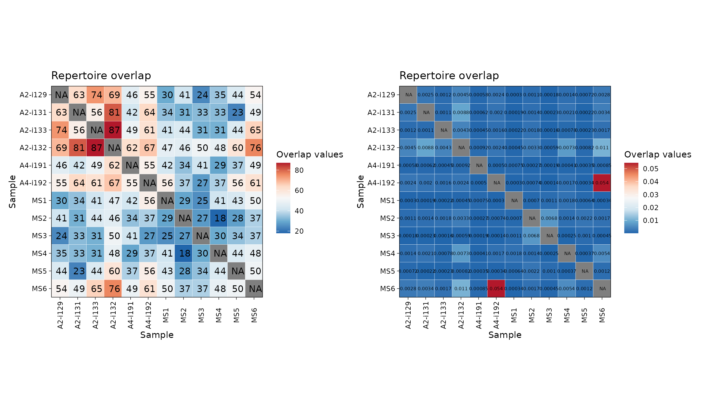
vis(imm_ov1, "heatmap2")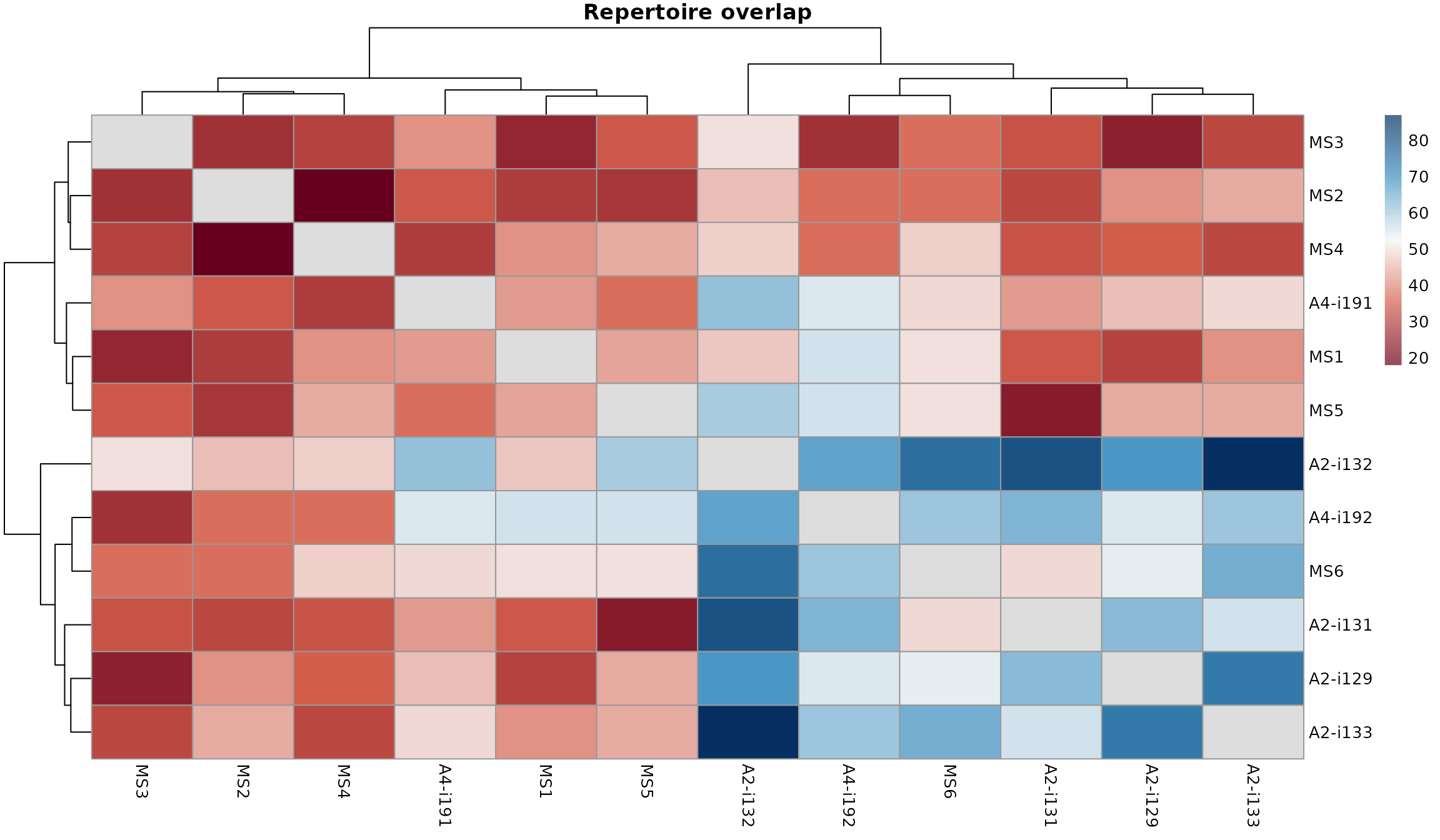
You can easily change the number of significant digits:
p1 <- vis(imm_ov2, .text.size = 2.5, .signif.digits = 1)
p2 <- vis(imm_ov2, .text.size = 2, .signif.digits = 2)

p1 + p2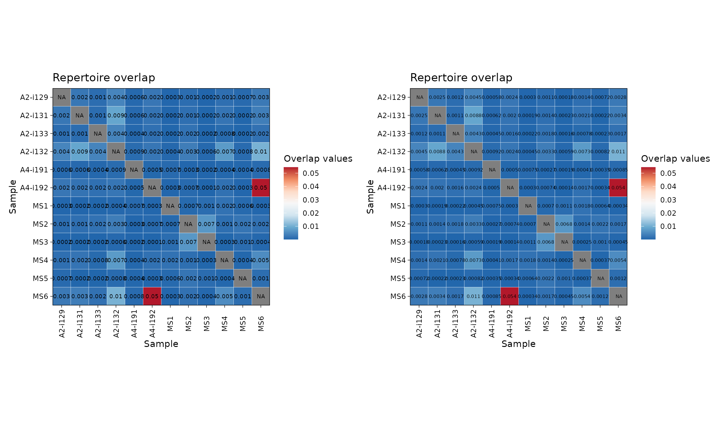
To analyse the computed overlap measures function apply repOverlapAnalysis.
# Apply different analysis algorithms to the matrix of public clonotypes:
# "mds" - Multi-dimensional Scaling
repOverlapAnalysis(imm_ov1, "mds")
## Standard deviations (1, .., p=4):
## [1] 0 0 0 0
##
## Rotation (n x k) = (12 x 2):
## [,1] [,2]
## A2-i129 -18.7767715 -18.360817
## A2-i131 29.9586985 -7.870441
## A2-i133 28.1148594 22.629093
## A2-i132 -44.3435640 6.221812
## A4-i191 13.8586515 7.452149
## A4-i192 -14.0065477 27.068830
## MS1 -8.8469009 -8.151574
## MS2 -0.9712073 -1.297017
## MS3 -10.4398629 4.894354
## MS4 0.5131505 10.471309
## MS5 18.5153823 -12.628029
## MS6 6.4241122 -30.429669
# "tsne" - t-Stochastic Neighbor Embedding
repOverlapAnalysis(imm_ov1, "tsne")
## DimI DimII
## A2-i129 -14.681797 51.77497
## A2-i131 -93.534895 -382.79904
## A2-i133 9.120198 98.58335
## A2-i132 79.226416 76.74444
## A4-i191 57.226722 121.18116
## A4-i192 -39.119764 74.22493
## MS1 -42.901807 40.28360
## MS2 62.099762 88.36805
## MS3 -26.670577 56.65753
## MS4 56.186325 100.61119
## MS5 -81.158822 -381.72072
## MS6 34.208239 56.09054
## attr(,"class")
## [1] "immunr_tsne" "matrix" "array"
# Visualise the results
repOverlapAnalysis(imm_ov1, "mds") %>% vis()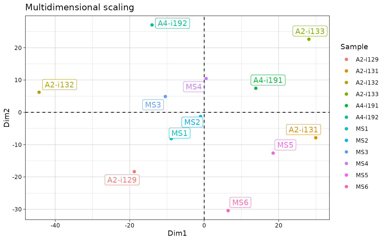
# Apply different analysis algorithms to the matrix of public clonotypes:
# "mds" - Multi-dimensional Scaling
repOverlapAnalysis(imm_ov1, "mds")
## Standard deviations (1, .., p=4):
## [1] 0 0 0 0
##
## Rotation (n x k) = (12 x 2):
## [,1] [,2]
## A2-i129 -18.7767715 -18.360817
## A2-i131 29.9586985 -7.870441
## A2-i133 28.1148594 22.629093
## A2-i132 -44.3435640 6.221812
## A4-i191 13.8586515 7.452149
## A4-i192 -14.0065477 27.068830
## MS1 -8.8469009 -8.151574
## MS2 -0.9712073 -1.297017
## MS3 -10.4398629 4.894354
## MS4 0.5131505 10.471309
## MS5 18.5153823 -12.628029
## MS6 6.4241122 -30.429669
# "tsne" - t-Stochastic Neighbor Embedding
repOverlapAnalysis(imm_ov1, "tsne")
## DimI DimII
## A2-i129 -90.06260 -184.739395
## A2-i131 114.12009 532.608800
## A2-i133 119.66661 -4.014284
## A2-i132 11.00240 -14.521507
## A4-i191 98.16866 -89.798868
## A4-i192 -141.65503 -224.506508
## MS1 -152.22429 -151.248953
## MS2 40.08289 -47.415057
## MS3 -117.80438 -181.995086
## MS4 67.65468 -57.386308
## MS5 87.73271 528.786357
## MS6 -36.68174 -105.769193
## attr(,"class")
## [1] "immunr_tsne" "matrix" "array"
# Visualise the results
repOverlapAnalysis(imm_ov1, "mds") %>% vis()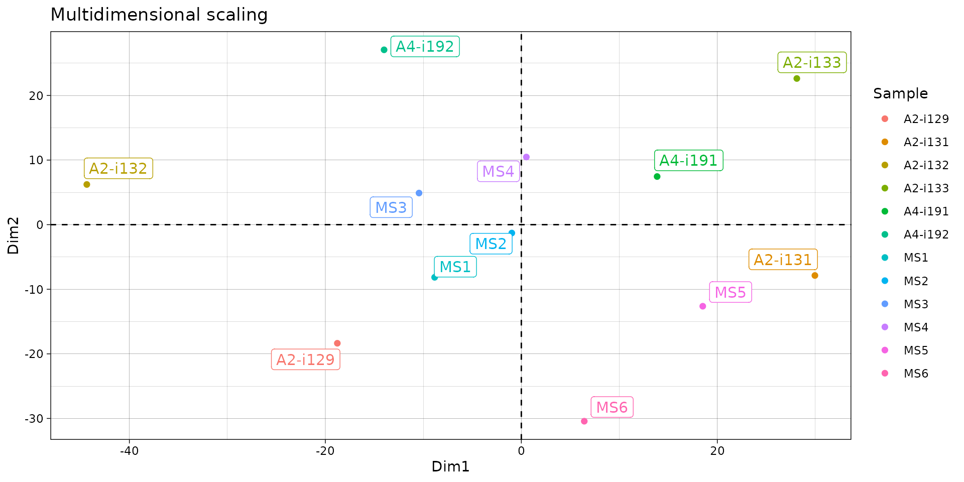
# Clusterise the MDS resulting components using K-means
repOverlapAnalysis(imm_ov1, "mds+kmeans") %>% vis()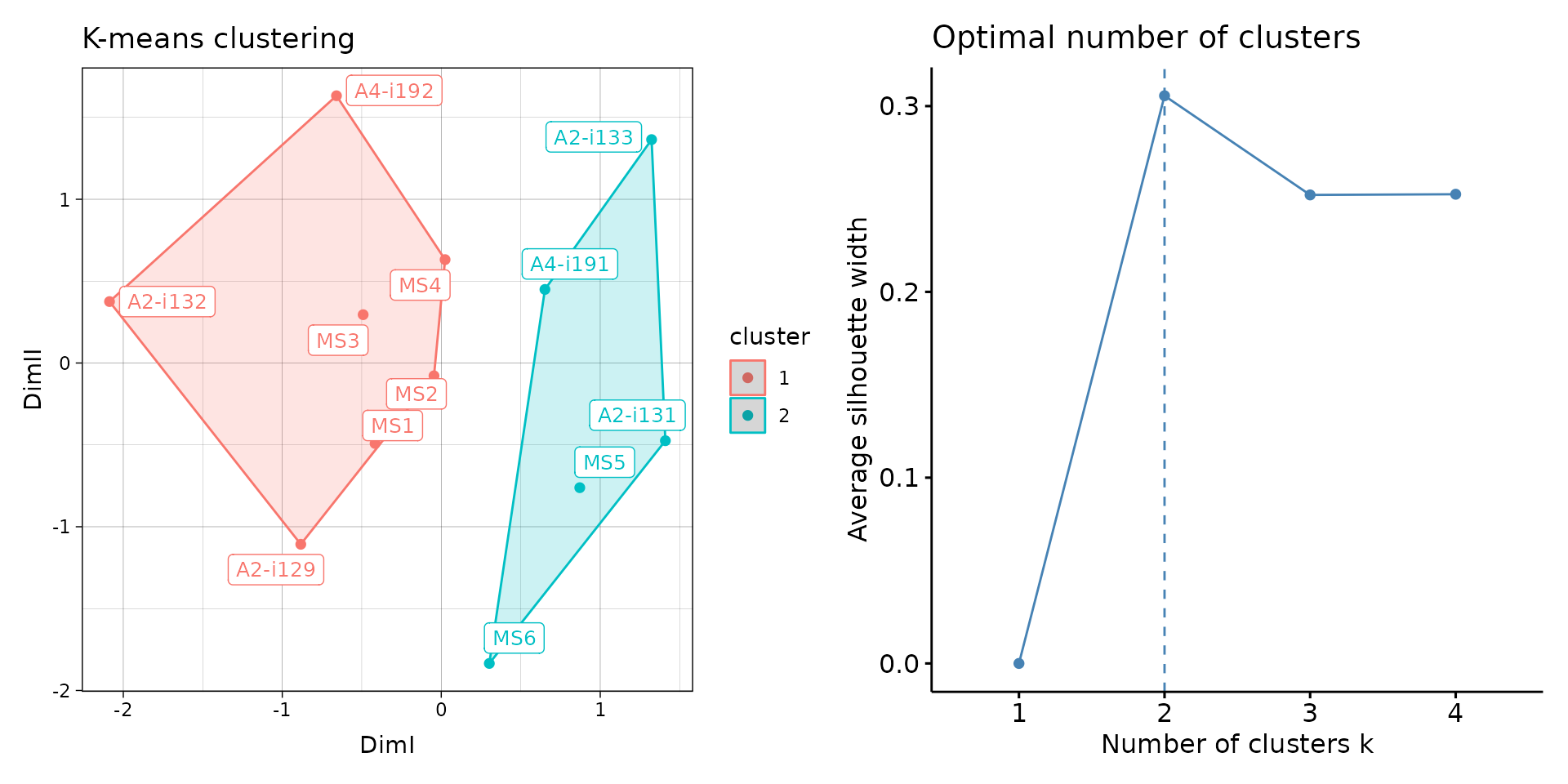
Public repertoire
In order to build a massive table with all clonotypes from the list of repertoires use the pubRep function.
# Pass "nt" as the second parameter to build the public repertoire table using CDR3 nucleotide sequences
pr.nt <- pubRep(immdata$data, "nt", .verbose = F)
pr.nt
## CDR3.nt Samples A2-i129
## 1: TGCGCCAGCAGCTTGGAAGAGACCCAGTACTTC 8 1
## 2: TGTGCCAGCAGCTTCCAAGAGACCCAGTACTTC 7 NA
## 3: TGTGCCAGCAGTTACCAAGAGACCCAGTACTTC 7 1
## 4: TGCGCCAGCAGCTTCCAAGAGACCCAGTACTTC 6 2
## 5: TGTGCCAGCAGCCAAGAGACCCAGTACTTC 6 4
## ---
## 75101: TGTGCTTCACAACTCTTATTGGACGAGACCCAGTACTTC 1 NA
## 75102: TGTGCTTCACAAGCCCTACAGGGCACTTTCCATAATTCACCCCTCCACTTT 1 NA
## 75103: TGTGCTTCAGGGCGGGCCTACGAGCAGTACTTC 1 NA
## 75104: TGTGCTTCCGCCGGACCGGACCGGGAGACCCAGTACTTC 1 NA
## 75105: TGTGCTTGCGGGACAGATAACTATGGCTACACCTTC 1 NA
## A2-i131 A2-i133 A2-i132 A4-i191 A4-i192 MS1 MS2 MS3 MS4 MS5 MS6
## 1: NA 1 1 NA 1 NA NA 1 1 1 1
## 2: 1 1 2 1 NA 1 NA NA 2 NA 1
## 3: 1 1 NA 1 1 1 NA 2 NA NA NA
## 4: NA 1 1 NA NA NA 1 NA 1 NA 1
## 5: 2 NA 2 3 1 NA NA NA NA 4 NA
## ---
## 75101: 1 NA NA NA NA NA NA NA NA NA NA
## 75102: NA NA NA NA NA NA NA NA NA 1 NA
## 75103: NA NA NA NA NA 1 NA NA NA NA NA
## 75104: NA 1 NA NA NA NA NA NA NA NA NA
## 75105: NA NA NA NA 1 NA NA NA NA NA NA
# Pass "aa+v" as the second parameter to build the public repertoire table using CDR3 aminoacid sequences and V alleles
# In order to use only CDR3 aminoacid sequences, just pass "aa"
pr.aav <- pubRep(immdata$data, "aa+v", .verbose = F)
pr.aav
## CDR3.aa V.name Samples A2-i129 A2-i131 A2-i133 A2-i132
## 1: CASSLEETQYF TRBV5-1 8 1 NA 2 1
## 2: CASSDSSGGANEQFF TRBV6-4 6 1 1 2 NA
## 3: CASSFQETQYF TRBV5-1 6 3 NA 1 1
## 4: CASSLGETQYF TRBV12-4 6 2 NA NA 4
## 5: CASSDSGGSYNEQFF TRBV6-4 5 NA NA NA 3
## ---
## 74440: CTSSRPTQGAYEQYF TRBV7-2 1 NA NA NA NA
## 74441: CTSSSRAGAGTDTQYF TRBV7-2 1 NA NA NA NA
## 74442: CTSSYPGLAGLKRKETQYF TRBV7-2 1 NA NA NA 1
## 74443: CTSSYRQRPYQETQYF TRBV7-2 1 NA NA NA NA
## 74444: CTSSYSTSGVGQFF TRBV7-2 1 NA NA NA NA
## A4-i191 A4-i192 MS1 MS2 MS3 MS4 MS5 MS6
## 1: NA 2 NA NA 1 1 1 1
## 2: 3 NA NA NA 2 NA NA 12
## 3: NA NA NA 1 NA 1 NA 1
## 4: 3 NA 1 NA NA NA 2 1
## 5: NA 1 1 NA 1 NA NA 1
## ---
## 74440: NA NA NA NA NA NA NA 1
## 74441: NA NA NA NA 1 NA NA NA
## 74442: NA NA NA NA NA NA NA NA
## 74443: NA NA NA NA 1 NA NA NA
## 74444: NA NA NA NA NA 1 NA NA
# You can also pass the ".coding" parameter to filter out all noncoding sequences first:
pr.aav.cod <- pubRep(immdata$data, "aa+v", .coding = T)
# Create a public repertoire with coding-only sequences using both CDR3 amino acid sequences and V genes
pr <- pubRep(immdata$data, "aa+v", .coding = T, .verbose = F)

# Apply the filter subroutine to leave clonotypes presented only in healthy individuals
pr1 <- pubRepFilter(pr, immdata$meta, c(Status = "C"))

# Apply the filter subroutine to leave clonotypes presented only in diseased individuals
pr2 <- pubRepFilter(pr, immdata$meta, c(Status = "MS"))

# Divide one by another
pr3 <- pubRepApply(pr1, pr2)

# Plot it
p <- ggplot() +
  geom_jitter(aes(x = "Treatment", y = Result), data = pr3)
p