BCR

Overview

A B-cell receptor (BCR) consists of an immunoglobulin molecule and a СD79 molecule. BCR includes two identical heavy chains (generated by recombination of V, D, and J segments), and two identical light chains (generated by recombination of V and J segments). Rapid improvements in high-throughput sequencing provide an opportunity to study B-cell immunoglobulin receptors on the cell surface [1] via the process called BCR repertoire sequencing. This pipeline describes how to work with BCR repertoire data after preprocessing raw sequenced data with MiXCR (https://docs.milaboratories.com/mixcr/about/) or any other programs.

The pipeline involves five steps:

Data loading.

The step includes loading the data and checking whether there is enough information for the pipeline to work.
Reconstructing clonal lineages.

At this step, all BCR sequences are divided into clonal lineages — sets of sequences that presumably share a common ancestor.
Building germline.

At this step, the algorithm generates a sequence that represents the ancestral sequence for each BCR in a clonal lineage.
Aligning sequences within clonal lineages.

This step involves preparation for phylogenetic and somatic hypermutation analysis.
Phylogenetic analysis.

This step provides phylogeny reconstruction and trunk length calculation (by running the PHYLIP package).
Somatic hypermutation analysis.

At this step, we compare clonotype and germline sequences to detect and count the number of mutations in clonotype sequence.

Data loading

BCR data are loaded with repLoad functions, like any other data.

Check that BCR data has the following:

information about full sequence read of each BCR,
positions of CDR3 region start and end,
number of mutations per CDR3 region. In MiXCR output files, this information is located in the column ‘refPoints’

Look at the sample BCR data implemented in Immunarch:

#load the package into the R environment:
library(immunarch)

data(bcrdata)

Reconstructing clonal lineages

B-cell clonal lineage represents a set of B cells that presumably have a common origin (arising from the same VDJ rearrangement event) and a common ancestor. BCR sequences are clustered according to their similarity, and sets of sequences in one cluster are named clonal lineages. Clustering involves two steps.

The first step is calculating the distance between sequences.
The second step is clustering the sequences using the information about the distance between them. Check our tutorial for more information about clustering: https://immunarch.com/articles/web_only/clustering.html

An example of reconstructing clonal lineages using default Immunarch options:

#calulate distance matrix
distBCR <- seqDist(bcrdata$data %>% top(500))

#find clusters
bcrdata$data <- seqCluster(bcrdata$data %>% top(500), distBCR, .perc_similarity = 0.9)

## Warning: There was 1 warning in `mutate()`.
## ℹ In argument: `length_value = map_chr(.y, ~ifelse(all(.x == .x[1]), yes =
##   .x[1], no = glue("range_{min(.x)}:{max(.x)}")))`.
## Caused by warning:
## ! Automatic coercion from integer to character was deprecated in purrr 1.0.0.
## ℹ Please use an explicit call to `as.character()` within `map_chr()` instead.
## ℹ The deprecated feature was likely used in the immunarch package.
##   Please report the issue at <https://github.com/immunomind/immunarch/issues>.

Building germline

Each clonal lineage has its own germline sequence that represents the ancestral sequence for each BCR in the clonal lineage. In other words, germline sequence is a sequence of B-cells immediately after VDJ recombination, before B-cell maturation and hypermutation process. Germline sequence is useful for assessing the degree of mutation and maturity of the repertoire.

In Immunarch, repGermline() function generates germline for each sequence:

#generate germline
bcrdata$data %>%
    repGermline(.threads = 1)

A germline is represented via sequences of V gene - N…N (CDR3 length) - J gene:

#germline example
bcrdata$data %>%
     top(1) %>%
     repGermline(.threads = 1) %>% .$full_clones %>% .$Germline.sequence

## [1] "CAGCTGCAGCTGCAGGAGTCGGGCCCAGGACTGGTGAAGCCTTCGGAGACCCTGTCCCTCACCTGCACTGTCTCTGGTGGCTCCATCAGCAGTAGTAGTTACTACTGGGGCTGGATCCGCCAGCCCCCAGGGAAGGGGCTGGAGTGGATTGGGAGTATCTATTATAGTGGGAGCACCTACTACAACCCGTCCCTCAAGAGTCGAGTCACCATATCCGTAGACACGTCCAAGAACCAGTTCTCCCTGAAGCTGAGCTCTGTGACCGCCGCAGACACGGCTGTGTATTACNNNNNNNNNNNNNNNNNNNNNNNNNNNNNNNNNNNNNNNGGCCAAGGAACCCTGGTCACCGTCTCCTCAG"

Оptions:

.data - The data to be processed. Can be data.frame, data.table, or a list of these objects.

.species - Specifies species from which reference V and J are taken. Available species: “HomoSapiens” (default), “MusMusculus”, “BosTaurus”, “CamelusDromedarius”, “CanisLupusFamiliaris”, “DanioRerio”, “MacacaMulatta”, “MusMusculusDomesticus”, “MusMusculusCastaneus”, “MusMusculusMolossinus”, “MusMusculusMusculus”, “MusSpretus”, “OncorhynchusMykiss”, “OrnithorhynchusAnatinus”, “OryctolagusCuniculus”, “RattusNorvegicus”, “SusScrofa”.

.min_nuc_outside_cdr3 - This parameter sets how many nucleotides should have V or J chain outside of CDR3 to be considered good for further alignment. Reads with too short chains are filtered out.

.threads - The number of threads to use.

Aligning sequences within a clonal lineage

After building clonal lineage and germline, we can start analyzing the degree of mutation and maturity of each clonal lineage. This allows us to find cells with a large number of mutated clones. The phylogenetic analysis will find mutations that influence the affinity of BCRs. Aligning the sequence is the first step toward sequence phylogenetic analysis.

In the Immunarch package, the function repAlignLineage aligns sequences within clonal lineages. This function requires Clustal W app to be installed. The app could be downloaded here: http://www.clustal.org/download/current/, or installed via your system package manager (such as apt or dnf).

For Ubuntu, check this guide: https://www.howtoinstall.me/ubuntu/18-04/clustalw/

sudo apt update
sudo apt install clustalw

For Windows, download and run clustalw-x.x-win.msi

repAlignLineage usage example:

data(bcrdata)
bcr_data <- bcrdata$data %>% top(500)
bcr_data %>%
  seqCluster(seqDist(bcr_data), .fixed_threshold = 3) %>%
  repGermline(.threads = 1) %>%
  repAlignLineage(.min_lineage_sequences = 2)

The function has several parameters:

.min_lineage_sequences — Filters clusters (clonal lineages) with the number of clonotypes lower than the threshold. Aligning clonal lineages with few sequences is of little use.

# take clusters that contain at least 1 sequence
bcr_data <- bcrdata$data
align_dt <- bcr_data %>%
  seqCluster(seqDist(bcr_data, .col = 'CDR3.nt', .group_by_seqLength = TRUE),
             .perc_similarity = 0.6) %>%
  repGermline(.threads = 1) %>%
  repAlignLineage(.min_lineage_sequences = 6, .align_threads = 2, .nofail = TRUE)

## Warning in merge_reference_sequences(., reference, "V", species, sample_name): Genes or alleles IGHV4-55 from sample full_clones not found in the reference and will be dropped!
## Probably, species argument is wrong (current value: HomoSapiens) or the data contains non-BCR genes.

.prepare_threads — the number of threads to prepare results table. A high number can cause memory overload!
.align_threads — the number of threads for lineage alignment.

Requirements for the input table for repAlignLineage()

must have columns in the immunarch compatible format immunarch_data_format,
must contain the ‘Cluster’ column generated by seqCluster() function,
must contain the ‘Sequence.germline’ column generated by repGermline() function.

Align sequences in a cluster can be visualized using standard functions:

# A name of the first cluster
align_dt$full_clones$Cluster[[1]]

## [1] "IGHV1-69/IGHJ6_length_63_cluster_1"

# Alignment of sequences from the first cluster
image(align_dt$full_clones$Alignment[[1]], grid = TRUE)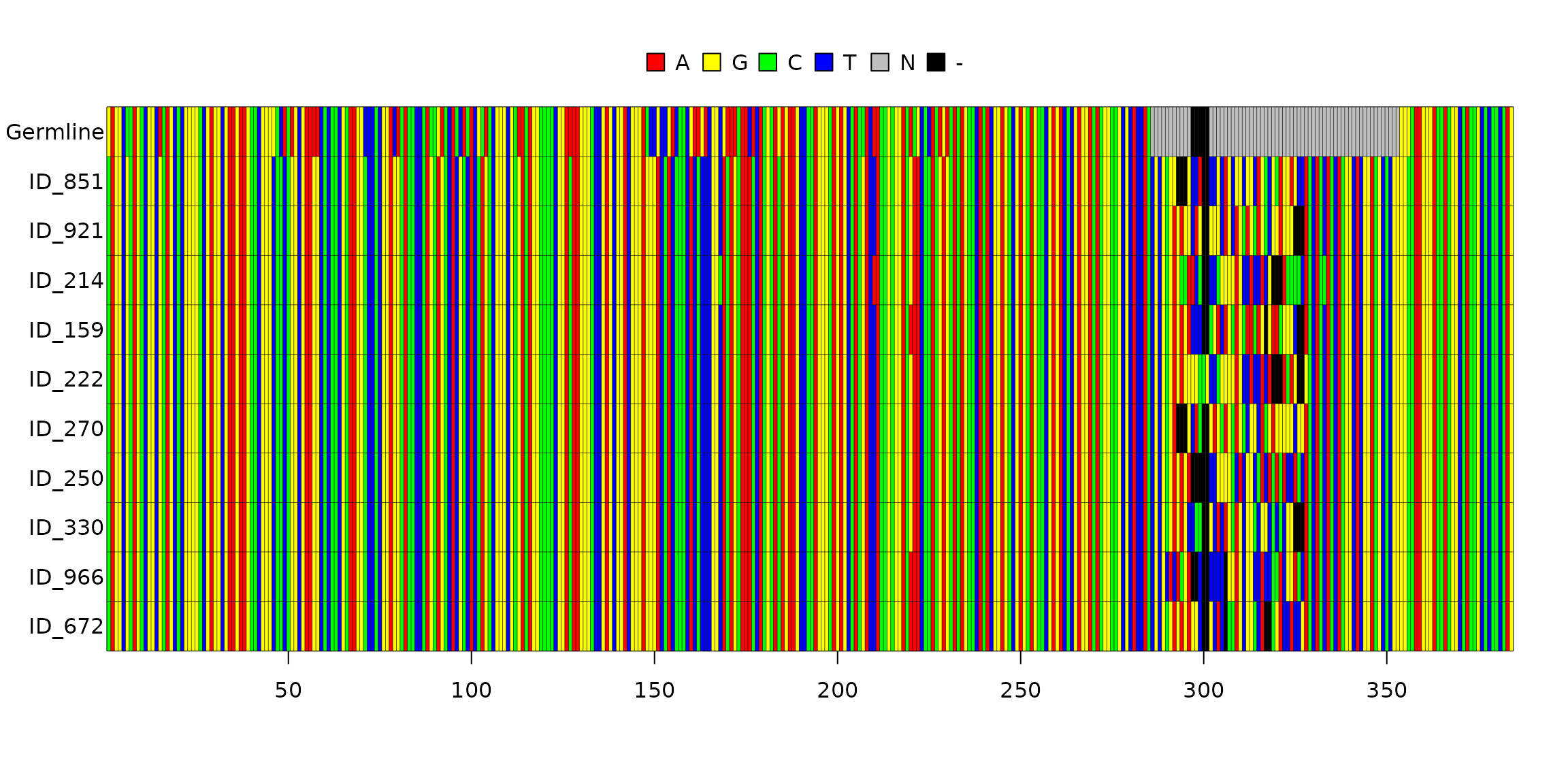

Phylogenetic analysis

For BCR phylogenetic analysis, we use the maximum parsimony method. The maximum parsimony method reconstructs a phylogenetic tree for the lineage by minimizing the total number of mutation events [2].

This method also enables the reconstruction of intermediate sequences that may have existed between BCR and germline sequence. These simulated sequences contain mutations that were ancestral to the clonotype group selected with the maximum parsimony analysis.

In Immunarch, function repClonalFamily builds a phylogeny of B-cells, generates a common ancestor, and calculates a trunk length. The mean trunk length represents the distance between the most recent common ancestor and germline sequence [3]. Mean trunk length serves as a measure of the maturity of a lineage. The trunk length of the lineage tree approximates the maturation state of the initiating B cell for each clone [4].

This function requires PHYLIP app to be installed. The app can be downloaded here: https://evolution.genetics.washington.edu/phylip/getme-new1.html, or could be installed with your system package manager (such as apt or dnf).

For Ubuntu, follow the installation guide (https://zoomadmin.com/HowToInstall/UbuntuPackage/phylip ):

sudo apt-get update -y
sudo apt-get install -y phylip

For Windows:
1. Download a Zip archive (https://evolution.genetics.washington.edu/phylip/install.html).
2. Extract the archive into a folder.
3. Add the folder to the PATH (https://www.architectryan.com/2018/03/17/add-to-the-path-on-windows-10/)

repClonalFamily usage example:

bcr <- align_dt %>%
  repClonalFamily(.threads = 2, .nofail = TRUE)
#plot visualization of the first tree
vis(bcr[["full_clones"]][["TreeStats"]][[1]])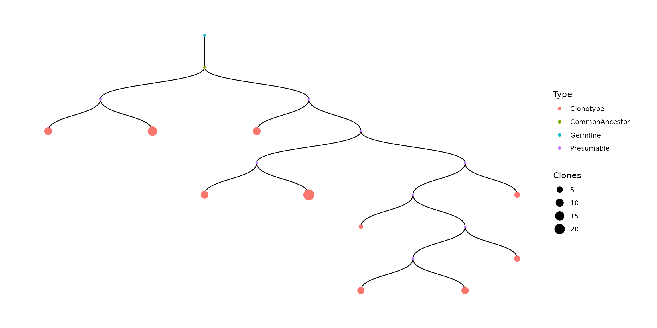

For each cluster tree is represented as table (The default number of clones for CommonAncestor, Germline, Presumable is 1):

#example for the first tree
bcr[["full_clones"]][["TreeStats"]][[1]]

You can recolor leaves. For example, we recolor leaves where number of AA mutations is not 0:

#take sequence where number of AA mutations is not 0
f <- bcr[["full_clones"]][["TreeStats"]][[1]]
#rename these leaves
f[f$DistanceAA != 0, ]['Type'] = 'mutationAA'
#new tree
vis(f)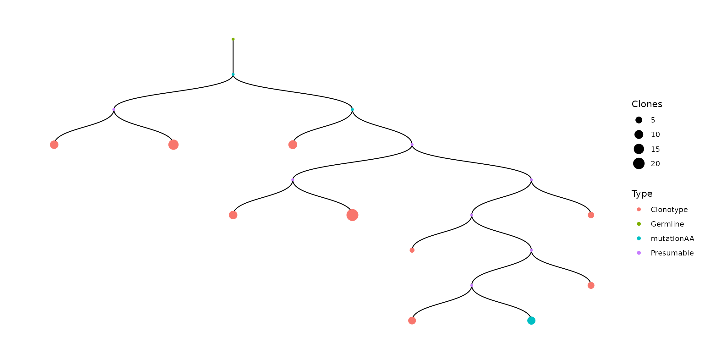

Another way to recolor leaves is to use .vis_groups parameter for repClonalFamily. It allows to assign group names for specific clone IDs, or lists of clone IDs:

#get all clone IDs from align_dt
clone_ids <- unnest(align_dt[["full_clones"]], "Sequences")[["Clone.ID"]]
#run repClonalFamily with assigning some of these clones to differently named and colored groups
bcr_with_groups <- align_dt %>%
  repClonalFamily(.vis_groups = list(
                    Group1 = clone_ids[1],
                    Group2 = clone_ids[3],
                    Group3 = list(clone_ids[5], clone_ids[2]),
                    Group4 = c(clone_ids[7], clone_ids[4])
                   ), .threads = 2, .nofail = TRUE
                 )
#display the first tree from repClonalFamily results
vis(bcr_with_groups[["full_clones"]][["TreeStats"]][[1]])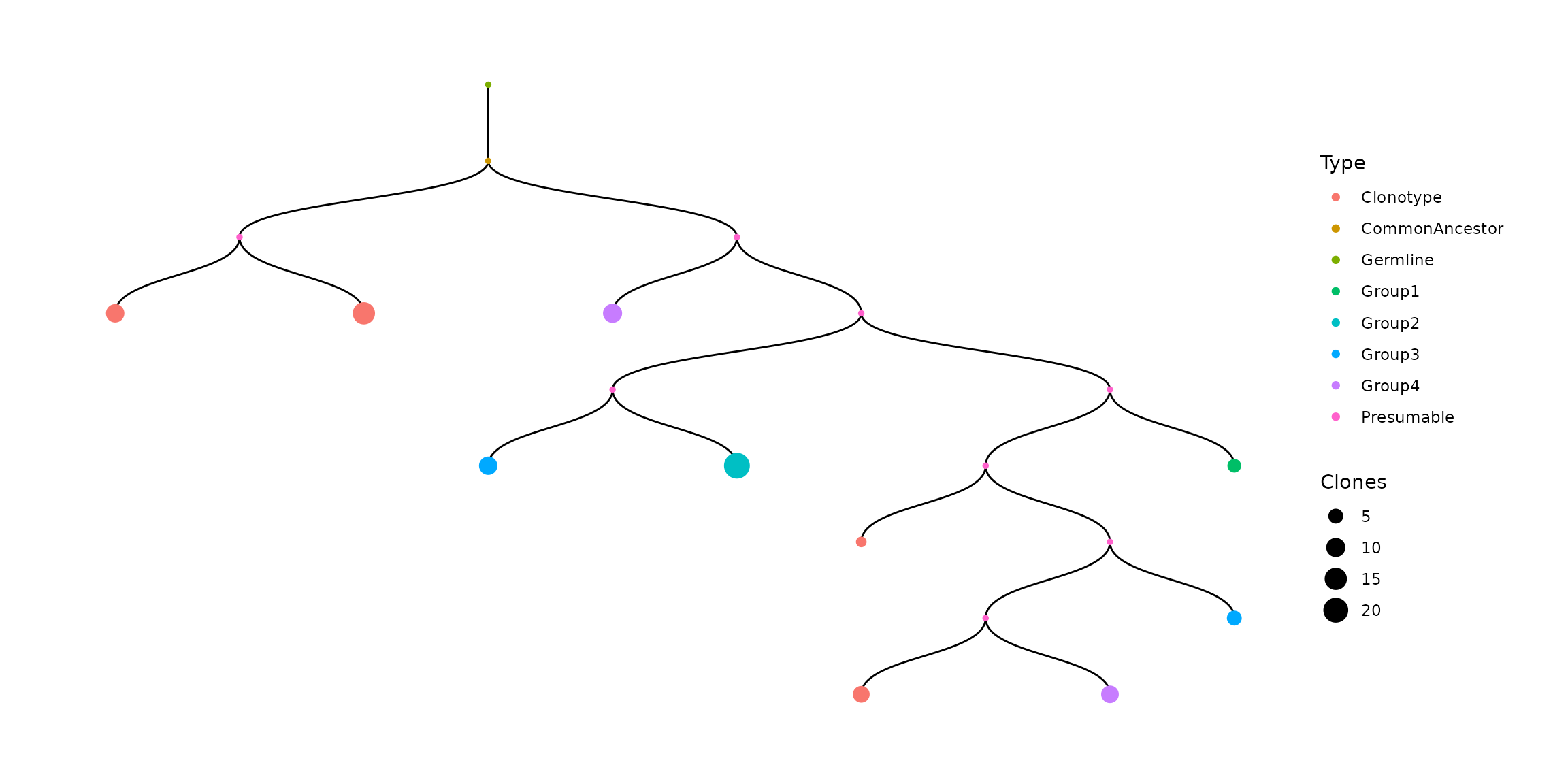

We have found 4 clusters:

bcr$full_clones$Cluster %>% unique()

## [1] "IGHV1-69/IGHJ6_length_63_cluster_1" "IGHV1-69/IGHJ6_length_75_cluster_2"
## [3] "IGHV3-23/IGHJ4_length_45_cluster_1" "IGHV3-23/IGHJ4_length_48_cluster_1"

We have found mismatches between a germline and an ancestor sequence. Dots represent nucleotides matches between the sequences, letters represent mismatches between the sequences:

# the example of common ancestor sequence
bcr$full_clones$Common.Ancestor[1]

## [1] "CAGGTGCAGCTGGTGCAGTCTGGGGCTGAGGTGAAGAAGCCTGGGTCCTCGGTGAAGGTCTCCTGCAAGGCTTCTGGAGGCACCTTCAGCAGCTATGCTATCAGCTGGGTGCGACAGGCCCCTGGACAAGGGCTTGAGTGGATGGGAGGGATCATCCCTATCTTTGGTACAGCAAACTACGCACAGAAGTTCCAGGGCAGAGTCACGATTACCGCGGACAAATCCACGAGCACAGCCTACATGGAGCTGAGCAGCCTGAGATCTGAGGACACGGCCGTGTATTACTGTGCGAGAGA-----TTDKGGCAGTGGTTATWCSMWKAACTACTACTACTACGGTATGGACGTCTGGGGCCAAGGGACCACGGTCACCGTCTCCTCAG"

# the example of mismatches between a germline and an ancestor sequence
bcr$full_clones$Germline.Output[1]

## [1] "GAGGTCCAGCTGGTACAGTCTGGGGCTGAGGTGAAGAAGCCTGGGGCTACAGTGAAAATCTCCTGCAAGGTTTCTGGATACACCTTCACCGACTACTACATGCACTGGGTGCAACAGGCCCCTGGAAAAGGGCTTGAGTGGATGGGACTTGTTGATCCTGAAGATGGTGAAACAATATACGCAGAGAAGTTCCAGGGCAGAGTCACCATAACCGCGGACACGTCTACAGACACAGCCTACATGGAGCTGAGCAGCCTGAGATCTGAGGACACGGCCGTGTATTACNNNNNNNNNNN-----NNNNNNNNNNNNNNNNNNNNNNNNNNNNNNNNNNNNNNNNNNNNNNNNNNNNGGGCAAGGGACCACGGTCACCGTCTCCTCAG"

We have calculated a trunk length for each cluster:

bcr$full_clones[ , c('Cluster', 'Trunk.Length') ]

##                              Cluster Trunk.Length
## 1 IGHV1-69/IGHJ6_length_63_cluster_1           52
## 2 IGHV1-69/IGHJ6_length_75_cluster_2           52
## 3 IGHV3-23/IGHJ4_length_45_cluster_1            2
## 4 IGHV3-23/IGHJ4_length_48_cluster_1            1

Also trunk length specified in “TreeStats” table in column “DistanceNT”.

#example fot first tree
bcr[["full_clones"]][["TreeStats"]][[1]][1, ]

Somatic hypermutation analysis

The rate of somatic hypermutation allows us to estimate repertoire maturation and detect the type of mutation contributing to the emergence of high affinity antibodies. This makes somatic hypermutation analysis a valuable asset for B-cell repertoire analysis.

In Immunarch, repSomaticHypermutation() function is designed for hypermutation analysis:

bcr_data <- bcrdata$data

shm_data <- bcr %>% repSomaticHypermutation(.threads = 2, .nofail = TRUE)

The function repSomaticHypermutation() takes V and J germline sequences and V and J clonotype sequences as an input. Then the function aligns germline and clonotype sequences to detect and calculate occurring mutations.

Examples of germline and clonotype sequences:

full_clones <- shm_data$full_clones
v_length <- nchar(paste(full_clones[1, "FR1.nt"], full_clones[1, "CDR1.nt"],
 full_clones[1, "FR2.nt"], full_clones[1, "CDR2.nt"], full_clones[1, "FR3.nt"], collapse=""))
j_length <- nchar(full_clones[1, "FR4.nt"])
seq_length <- nchar(full_clones[1, "Sequence"])

# the example of germline V sequence
full_clones$Germline.Input[1] %>% substr(1, v_length)

## [1] "GAGGTCCAGCTGGTACAGTCTGGGGCTGAGGTGAAGAAGCCTGGGGCTACAGTGAAAATCTCCTGCAAGGTTTCTGGATACACCTTCACCGACTACTACATGCACTGGGTGCAACAGGCCCCTGGAAAAGGGCTTGAGTGGATGGGACTTGTTGATCCTGAAGATGGTGAAACAATATACGCAGAGAAGTTCCAGGGCAGAGTCACCATAACCGCGGACACGTCTACAGACACAGCCTACATGGAGCTGAGCAGCCTGAGATCTGAGGACACGGCCGTGTATTACNNNN"

# the example of germline J sequence
full_clones$Germline.Input[1] %>% substr(seq_length - j_length, seq_length)

## [1] "NGGGCAAGGGACCACGGTCACCGTCTCCTCAG"

# the example of clonotype V sequence
full_clones$Sequence[1] %>% substr(1, v_length)

## [1] "CAGGTGCAGCTGGTGCAGTCTGGGGCTGAGGTGAAGAAGCCTGGGTCCTCGGTGAAGGTCTCCTGCAAGGCTTCTGGAGGCACCTTCAGCAGCTATGCTATCAGCTGGGTGCGACAGGCCCCTGGACAAGGGCTTGAGTGGATGGGAGGGATCATCCCTATCTTTGGTACAGCAAACTACGCACAGAAGTTCCAGGGCAGAGTCACGATTACCGCGGACGAATCCACGAGCACAGCCTACATGGAGCTGAGCAGCCTGAGATCTGAGGACACGGCCGTGTATTACTGTG"

# the example of clonotype J sequence
full_clones$Sequence[1] %>% substr(seq_length - j_length, seq_length)

## [1] "GGGCCAAGGGACCACGGTCACCGTCTCCTCAG"

Example: aligning germline and clonotype V sequences:

image(shm_data$full_clones$Germline.Alignment.V[[3]], grid = TRUE)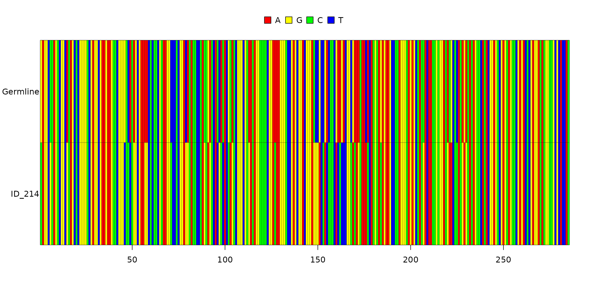

Example: aligning germline and clonotype J sequences:

image(shm_data$full_clones$Germline.Alignment.J[[3]], grid = TRUE)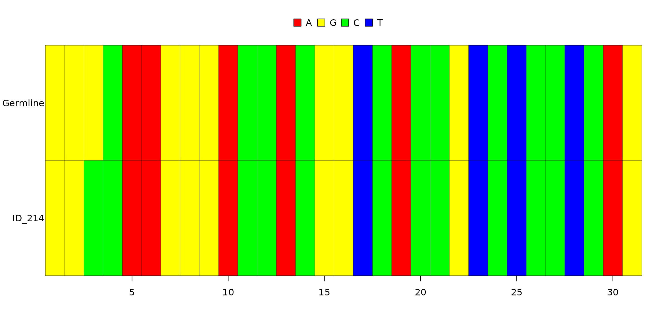

The number of mutations for each clonotype sequence:

cols <- c('Clone.ID', 'Substitutions', 'Insertions', 'Deletions', 'Mutations')
shm_data$full_clones[ , cols ]

##    Clone.ID Substitutions Insertions Deletions Mutations
## 1       851            53          0         0        53
## 2       921            53          0         0        53
## 3       214            53          0         0        53
## 4       159            52          0         0        52
## 5       222            53          0         0        53
## 6       270            53          0         0        53
## 7       250            53          0         0        53
## 8       330            53          0         0        53
## 9       966            52          0         0        52
## 10      672            52          0         0        52
## 11      401            53          0         0        53
## 12      386            53          0         0        53
## 13      736            53          0         0        53
## 14      295            53          0         0        53
## 15      202            53          0         0        53
## 16      716            52          0         0        52
## 17      827             1          0         0         1
## 18      591            16          0         0        16
## 19      433             1          0         0         1
## 20      163            22          0         0        22
## 21      914            24          0         0        24
## 22      524            12          0         0        12
## 23       24             6          0         0         6
## 24      342             6          0         0         6
## 25      940            19          0         0        19
## 26      238             6          0         0         6
## 27      428            15          0         0        15
## 28      484            13          0         0        13
## 29      932             1          0         0         1
## 30      517             4          0         0         4
## 31      522             4          0         0         4
## 32      933            12          0         0        12

Then you could easily estimate the mutation rate:

# estimate mutation rate
shm_data$full_clones %>%
  mutate(Mutation.Rate = Mutations / (nchar(Sequence) - nchar(CDR3.nt))) %>%
  select(Clone.ID, Mutation.Rate)

##    Clone.ID Mutation.Rate
## 1       851   0.167721519
## 2       921   0.167721519
## 3       214   0.167721519
## 4       159   0.164556962
## 5       222   0.167721519
## 6       270   0.167721519
## 7       250   0.167721519
## 8       330   0.167721519
## 9       966   0.164556962
## 10      672   0.164556962
## 11      401   0.167721519
## 12      386   0.167721519
## 13      736   0.167721519
## 14      295   0.167721519
## 15      202   0.167721519
## 16      716   0.164556962
## 17      827   0.003164557
## 18      591   0.050632911
## 19      433   0.003164557
## 20      163   0.069620253
## 21      914   0.075949367
## 22      524   0.037974684
## 23       24   0.018987342
## 24      342   0.018987342
## 25      940   0.060126582
## 26      238   0.018987342
## 27      428   0.047468354
## 28      484   0.041139241
## 29      932   0.003164557
## 30      517   0.012658228
## 31      522   0.012658228
## 32      933   0.037974684

ImmunoMind – improving design of T-cell therapies using multi-omics and AI. Research and biopharma partnerships, more details: immunomind.io

support@immunomind.io