![[Deprecated]](figures/lifecycle-deprecated.svg)
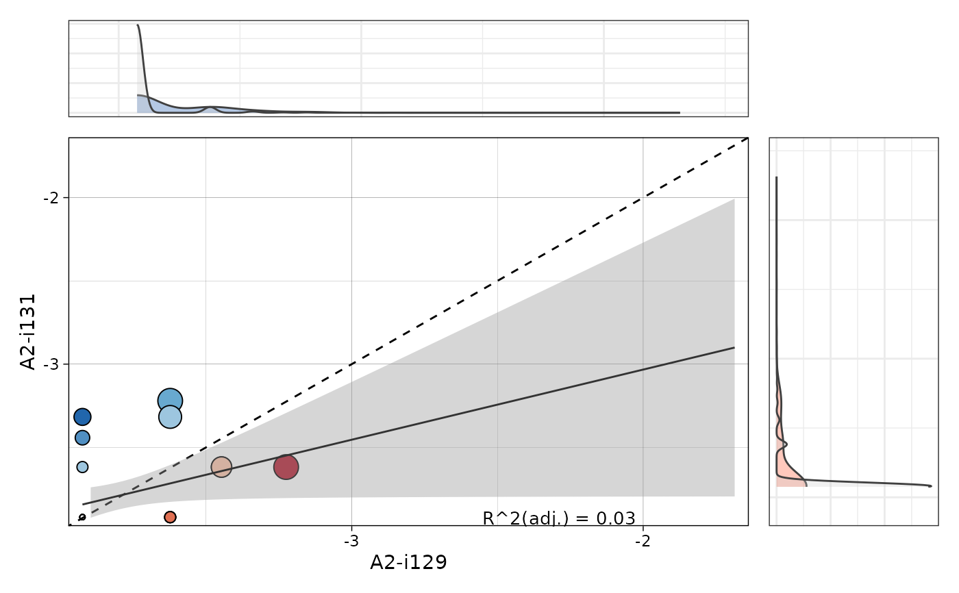
Visualise correlation of public clonotype frequencies in pairs of repertoires.
Usage
vis_public_clonotypes(
  .data,
  .x.rep = NA,
  .y.rep = NA,
  .title = NA,
  .ncol = 3,
  .point.size.modif = 1,
  .cut.axes = TRUE,
  .density = TRUE,
  .lm = TRUE,
  .radj.size = 3.5
)
Arguments
- .data
Public repertoire data - an output from the pubRep function.
- .x.rep
Either indices of samples or character vector of sample names for the x-axis. Must be of the same length as ".y.rep".
- .y.rep
Either indices of samples or character vector of sample names for the y-axis. Must be of the same length as ".x.rep".
- .title
The text for the title of the plot.
- .ncol
An integer number of columns to print in the grid of pairs of repertoires.
- .point.size.modif
An integer value that is a modifier of the point size. The larger the number, the larger the points.
- .cut.axes
If TRUE then axes limits become shorter.
- .density
If TRUE then displays density plot for distributions of clonotypes for each sample. If FALSE then removes density plot from the visualisation.
- .lm
If TRUE then fit a linear model and displays an R adjusted coefficient that shows how similar samples are in terms of shared clonotypes.
- .radj.size
An integer value, that defines the size of the The text for the R adjusted coefficient.