Basic analysis and clonality
ImmunoMind – improving design of T-cell therapies using multi-omics and AI. Research and biopharma partnerships, more details: immunomind.io
support@immunomind.io
Source:vignettes/web_only_v0/v3_basic_analysis.Rmd
v3_basic_analysis.RmdBasic analysis
For each task in this section immunarch includes
separate functions that are generally self-explanatory and are written
in CamelCase.
Note: all functions in immunarch require that the input immune
repertoire data list have names. If you use the repLoad
function, you will have no issues. If you compose your list by hand, you
must name elements in the list, e.g.:
your_data # Your list with repertoires without names

names(your_data)
# Output: NULL

names(your_data) <- sapply(1:length(your_data), function(i) paste0("Sample", i))
names(your_data)
# Output: Sample1 Sample2 ... Sample10
Basic analysis functions are:
repExplore- computes basic statistics, such as number of clones or distributions of lengths and counts. To explore them you need to pass the statistics, e.g.count, to the.method.repClonality- computes the clonality of repertoires.repOverlap- computes the repertoire overlap.repOverlapAnalysis- analyses the repertoire overlap, including different clustering procedures and PCA.geneUsage- computes the distributions of V or J genes.geneUsageAnalysis- analyses the distributions of V or J genes, including clustering and PCA.repDiversity- estimates the diversity of repertoires.trackClonotypes- analyses the dynamics of repertoires across time points.spectratype- computes spectratype of clonotypes.getKmersandkmer_profile- computes distributions of kmers and sequence profiles.
How to visualise analysis results
Output of each analysis function could be passed directly to the
vis function - the general function for visualisation.
Examples of usage are given below. Almost all visualisations of analysis
involves grouping data by their respective properties from the metadata
table or using user-supplied properties. Grouping is possible by passing
either .by argument or by passing both .by and
.meta arguments to the vis function.
- You can pass
.byas a character vector with one or several column names from the metadata table to group your data before plotting. In this case you should also provide the.metaargument with the metadata table.
exp_vol <- repExplore(immdata$data, .method = "volume")
p1 <- vis(exp_vol, .by = c("Status"), .meta = immdata$meta)
p2 <- vis(exp_vol, .by = c("Status", "Sex"), .meta = immdata$meta)
p1 + p2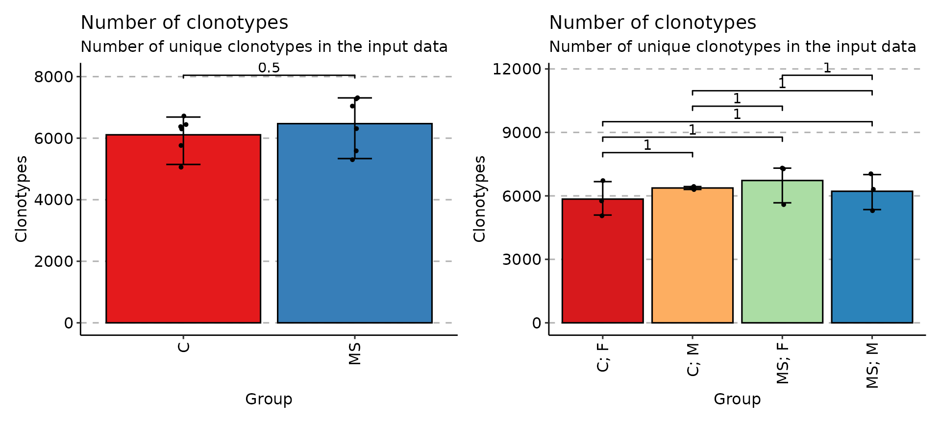
- You can pass
.byas a character vector that matches the number of samples in your data, each value should correspond to a sample’s property. It will be used to group data based on the values provided. Note that in this case you should pass NA to.meta.
exp_vol <- repExplore(immdata$data, .method = "volume")
by_vec <- c("C", "C", "C", "C", "C", "C", "MS", "MS", "MS", "MS", "MS", "MS")
p <- vis(exp_vol, .by = by_vec)
p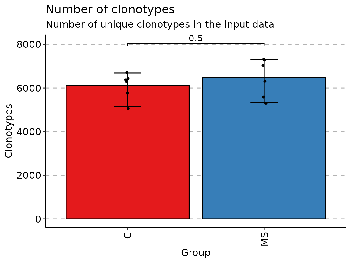
Once data is grouped, the statistical tests for comparing means of
groups will be performed, unless .test = F is supplied. In
case there are only two groups, the Wilcoxon
rank sum test is performed (R function wilcox.test with
an argument exact = F) for testing if there is a difference
in mean rank values between two groups. In case there more than two
groups, the Kruskal-Wallis
test is performed (R function kruskal.test), that is
equivalent to ANOVA for ranks and it tests whether samples from
different groups originated from the same distribution. A significant
Kruskal-Wallis test indicates that at least one sample stochastically
dominates one other sample. Adjusted for multiple comparisons P-values
are plotted on the top of groups. P-value adjusting is done using the Holm
method (also known as Holm-Bonferroni correction). You can execute
the command ?p.adjust in the R console to see more.
Plots generated by the vis function as well as any
ggplot2-based plots can be passed to fixVis—built-in
software tool for making publication-ready plots:
# 1. Analyse
exp_len <- repExplore(immdata$data, .method = "len", .col = "aa")

# 2. Visualise
p1 <- vis(exp_len)

# 3. Fix and make publication-ready results
fixVis(p1)
See the fixVis tutorial here.
Exploratory analysis
For the basic exploratory analysis such as comparing of number of
reads / UMIs per repertoire or distribution use the function
repExplore.
exp_len <- repExplore(immdata$data, .method = "len", .col = "aa")
exp_cnt <- repExplore(immdata$data, .method = "count")
exp_vol <- repExplore(immdata$data, .method = "volume")

p1 <- vis(exp_len)
p2 <- vis(exp_cnt)
p3 <- vis(exp_vol)

p1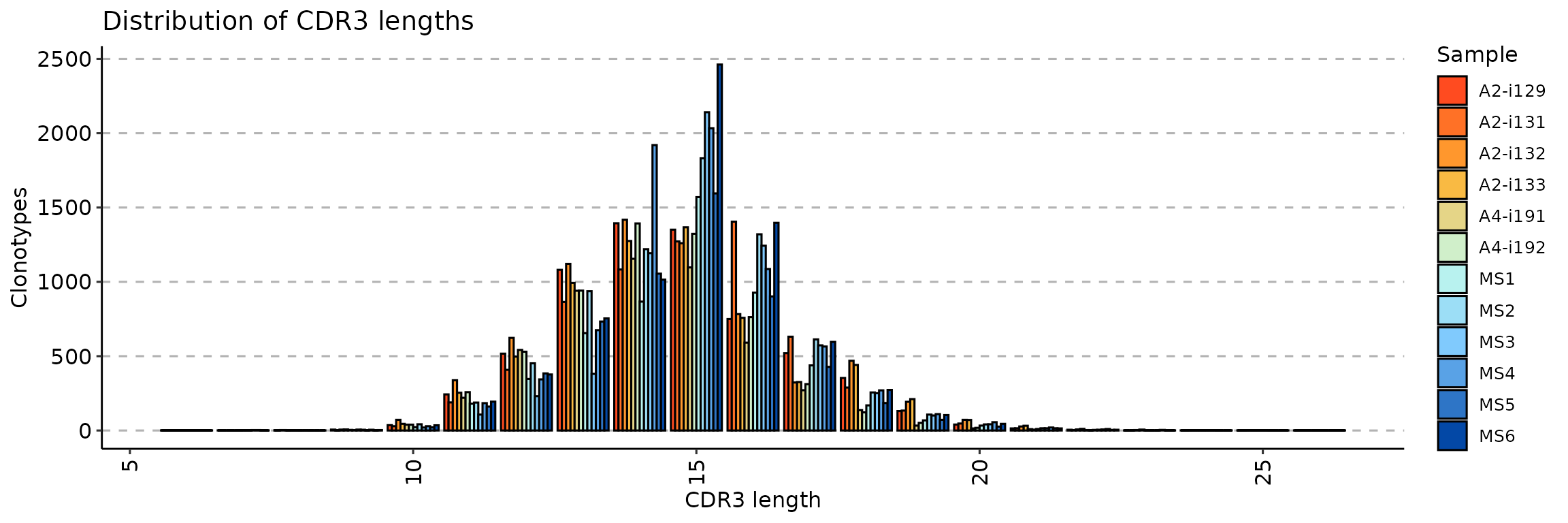
p2 + p3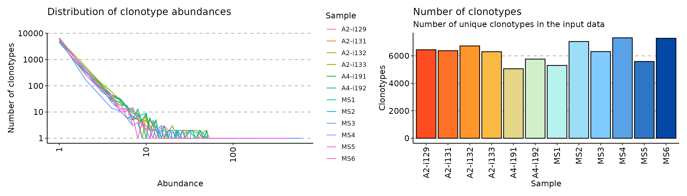
# You can group samples by their metainformation
p4 <- vis(exp_len, .by = "Status", .meta = immdata$meta)
p5 <- vis(exp_cnt, .by = "Sex", .meta = immdata$meta)
p6 <- vis(exp_vol, .by = c("Status", "Sex"), .meta = immdata$meta)

p4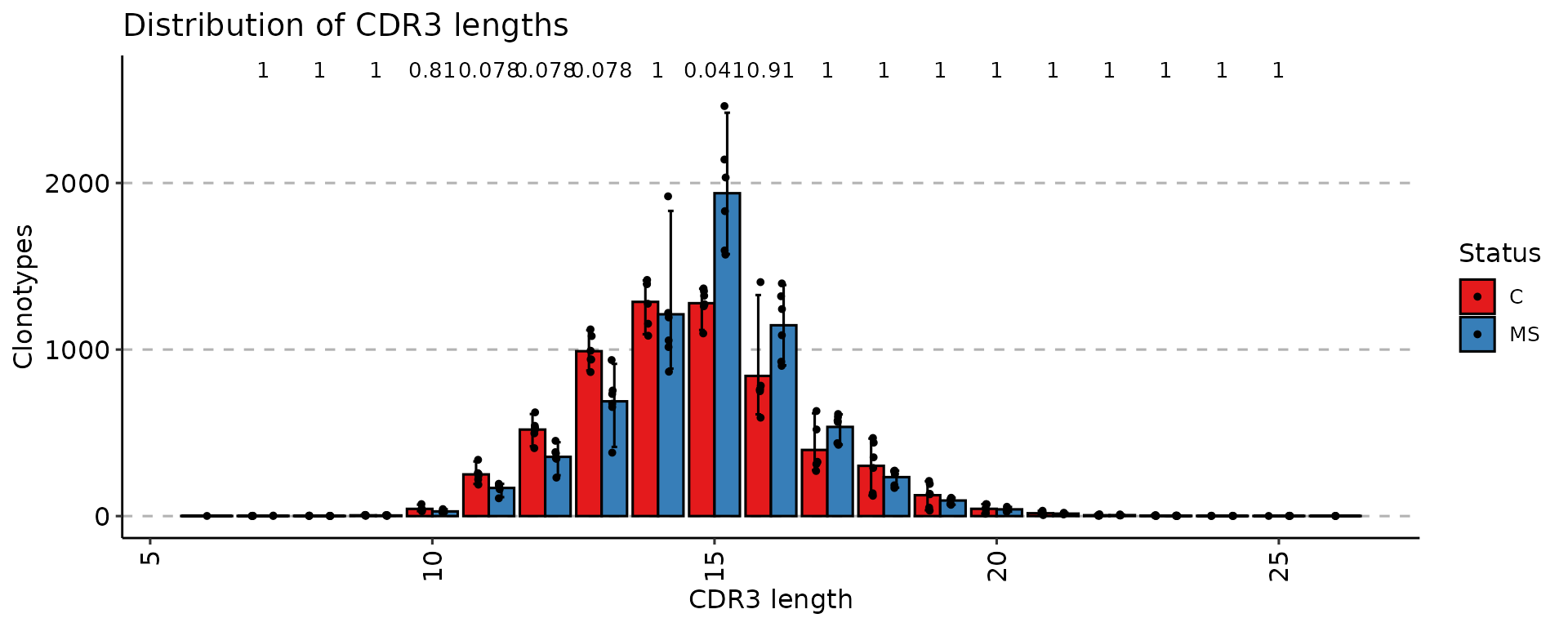
p5 + p6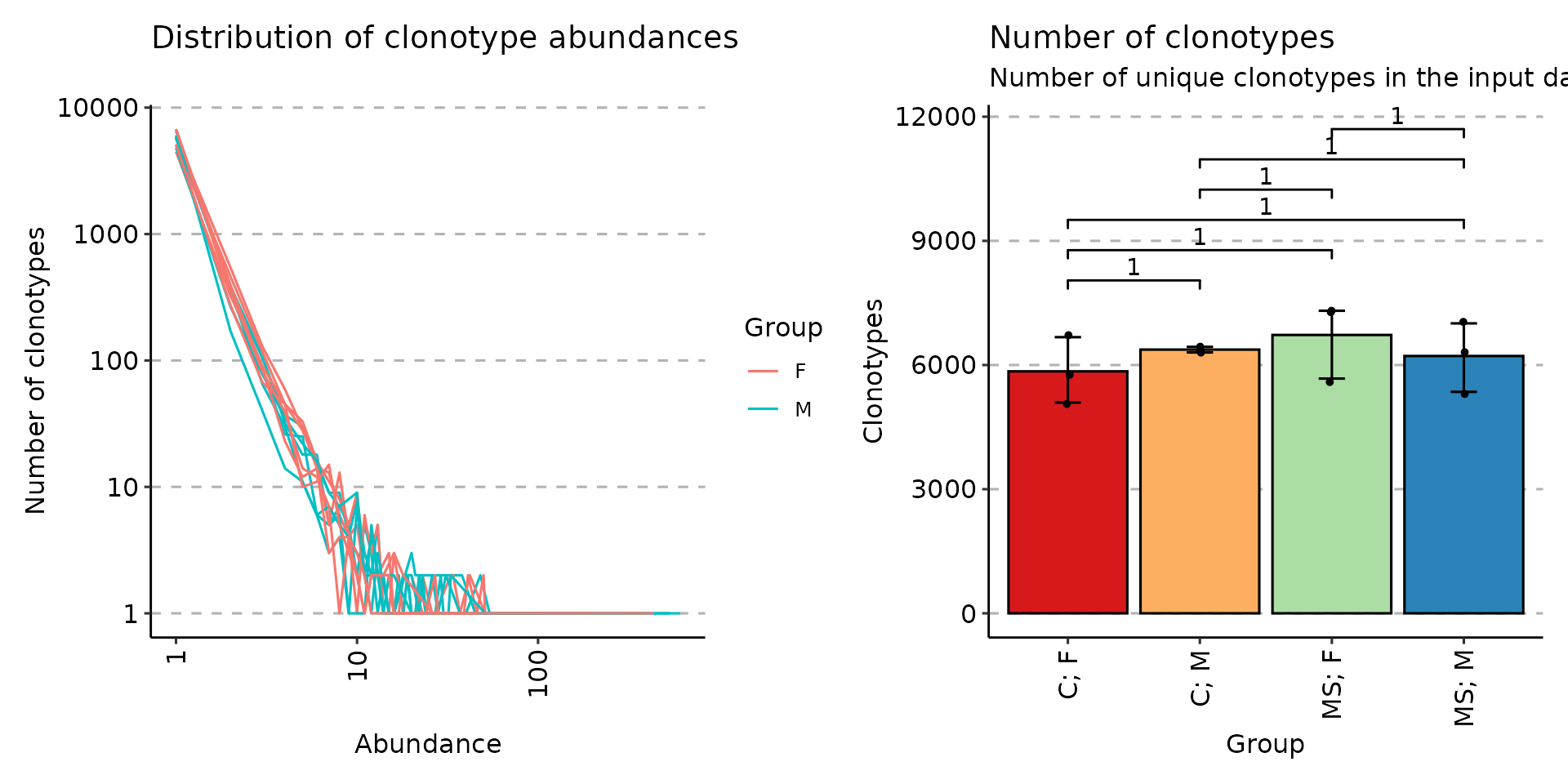
Clonality
One of the ways to estimate the diversity of samples is to evaluate
clonality. repClonality measures the amount of the most or
the least frequent clonotypes. There are several methods to assess
clonality, let us take a view of them. The clonal.prop
method computes the proportion of repertoire occupied by the pools of
cell clones:
imm_pr <- repClonality(immdata$data, .method = "clonal.prop")
imm_pr
## Clones Percentage Clonal.count.prop
## A2-i129 18 10.0 0.0027556644
## A2-i131 28 10.0 0.0042728521
## A2-i133 9 10.3 0.0014077898
## A2-i132 113 10.0 0.0164987589
## A4-i191 4 11.5 0.0007773028
## A4-i192 8 10.4 0.0013738623
## MS1 2 10.1 0.0003700278
## MS2 66 10.0 0.0092372288
## MS3 2 10.6 0.0003095496
## MS4 176 10.0 0.0236336780
## MS5 3 13.2 0.0005303164
## MS6 150 10.0 0.0202456472
## attr(,"class")
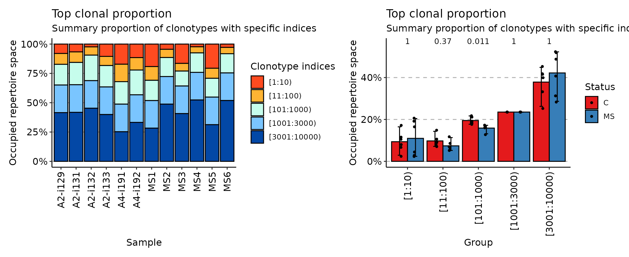
## [1] "immunr_clonal_prop" "matrix" "array"The top method considers the most abundant cell
clonotypes:
imm_top <- repClonality(immdata$data, .method = "top", .head = c(10, 100, 1000, 3000, 10000))
imm_top
## 10 100 1000 3000 10000
## A2-i129 0.08011765 0.17282353 0.3491765 0.5844706 1
## A2-i131 0.06670588 0.15647059 0.3467059 0.5820000 1
## A2-i133 0.10505882 0.18294118 0.3655294 0.6008235 1
## A2-i132 0.02388235 0.09423529 0.3118824 0.5471765 1
## A4-i191 0.17176471 0.32047059 0.5122353 0.7475294 1
## A4-i192 0.11541176 0.22141176 0.4325882 0.6678824 1
## MS1 0.19164706 0.30894118 0.4817647 0.7170588 1
## MS2 0.04458824 0.11470588 0.2770588 0.5123529 1
## MS3 0.16482353 0.23011765 0.3575294 0.5928235 1
## MS4 0.02329412 0.07517647 0.2415294 0.4768235 1
## MS5 0.20611765 0.29188235 0.4521176 0.6874118 1
## MS6 0.02835294 0.08235294 0.2460000 0.4812941 1
## attr(,"class")
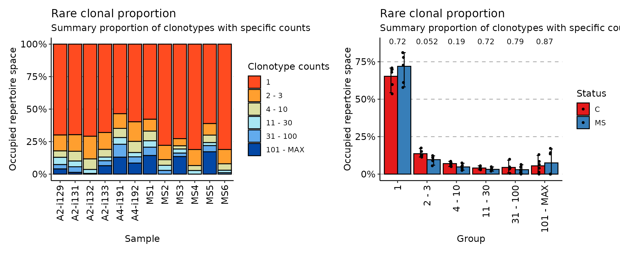
## [1] "immunr_top_prop" "matrix" "array"While the rare method deals with the least prolific
clonotypes:
imm_rare <- repClonality(immdata$data, .method = "rare")
imm_rare
## 1 3 10 30 100 MAX
## A2-i129 0.6991765 0.8215294 0.8710588 0.9267059 0.9604706 1
## A2-i131 0.6969412 0.8243529 0.8995294 0.9436471 0.9869412 1
## A2-i133 0.6800000 0.8100000 0.8690588 0.8974118 0.9357647 1
## A2-i132 0.7088235 0.8831765 0.9643529 0.9951765 1.0000000 1
## A4-i191 0.5355294 0.6484706 0.7189412 0.7707059 0.8697647 1
## A4-i192 0.5976471 0.7487059 0.8342353 0.8675294 0.9156471 1
## MS1 0.5780000 0.6692941 0.7438824 0.7929412 0.8571765 1
## MS2 0.7788235 0.8891765 0.9322353 0.9718824 1.0000000 1
## MS3 0.7272941 0.7825882 0.8071765 0.8385882 0.8652941 1
## MS4 0.8109412 0.9343529 0.9725882 1.0000000 1.0000000 1
## MS5 0.6112941 0.7001176 0.7575294 0.7809412 0.8284706 1
## MS6 0.8107059 0.9208235 0.9703529 0.9897647 1.0000000 1
## attr(,"class")
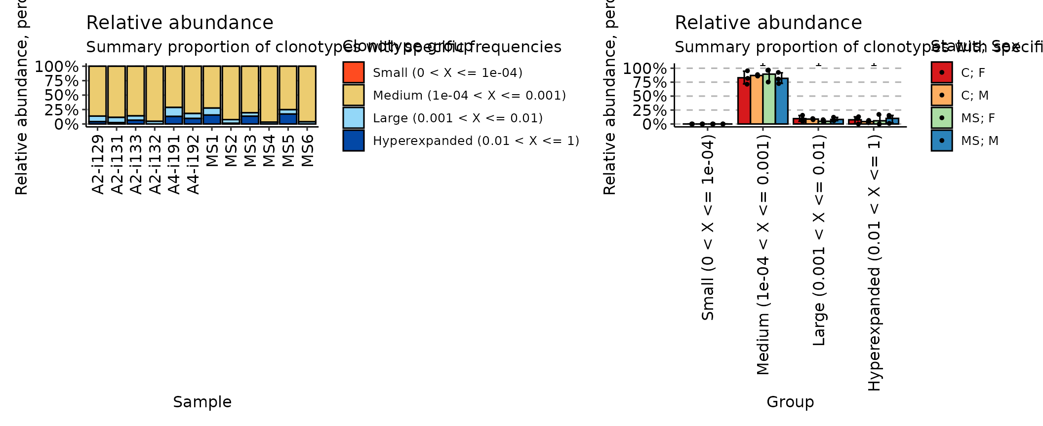
## [1] "immunr_rare_prop" "matrix" "array"Finally, the homeo method assesses the clonal space
homeostasis, i.e., the proportion of the repertoire occupied by the
clones of a given size:
imm_hom <- repClonality(immdata$data,
  .method = "homeo",
  .clone.types = c(Small = .0001, Medium = .001, Large = .01, Hyperexpanded = 1)
)
imm_hom
## Small (0 < X <= 1e-04) Medium (1e-04 < X <= 0.001)
## A2-i129 0 0.8634118
## A2-i131 0 0.8858824
## A2-i133 0 0.8597647
## A2-i132 0 0.9542353
## A4-i191 0 0.7135294
## A4-i192 0 0.8183529
## MS1 0 0.7248235
## MS2 0 0.9244706
## MS3 0 0.8061176
## MS4 0 0.9683529
## MS5 0 0.7520000
## MS6 0 0.9625882
## Large (0.001 < X <= 0.01) Hyperexpanded (0.01 < X <= 1)
## A2-i129 0.09705882 0.03952941
## A2-i131 0.09011765 0.02400000
## A2-i133 0.07600000 0.06423529
## A2-i132 0.04576471 0.00000000
## A4-i191 0.15623529 0.13023529
## A4-i192 0.08611765 0.09552941
## MS1 0.12082353 0.15435294
## MS2 0.06411765 0.01141176
## MS3 0.05917647 0.13470588
## MS4 0.03164706 0.00000000
## MS5 0.07647059 0.17152941
## MS6 0.03741176 0.00000000
## attr(,"class")
## [1] "immunr_homeo" "matrix" "array"